 Welcome to the Surrey Physics Plotters blog. It exists in the spirit of other blogs dedicated to the use of the gnuplot plotting program. While I don't consider myself as much of an expert at gnuplot as the writers of gnuplotting or gnuplot tricks, I think it would still be helpful to have another repository for useful examples that I, at least, will otherwise forget.
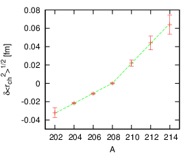
So - the first example comes in the form of a plot which includes a set of data defined at equally spaced points in the abscissa, whose ordinates show a sudden kink in the gradient (the data are the radii of a series of isotopes of lead nuclei - if you're interested, the paper is here).
I wanted to include on the plot a fit to the data, assuming one straight line up to atomic number 208, and a different straight line from 208 up. I'll show the code here, and explain how it works below.
set term postscript enhanced col size 10cm,8cm font 'Helvetica,12'The first two lines set up the output file as a postscript file (since this is what I wanted for the publication). Specifying the size here adds in the BoundingBox for encapsulated postscript, though it probably makes sense to use the eps option instead.
set out 'lead-exp.eps'
f1(x) = m1*(x-208)
f2(x) = m2*(x-208)
fit [202:208] f1(x) 'expdat.gnu' using 1:($2-5.5010):3 via m1
fit [208:214] f2(x) 'expdat.gnu' using 1:($2-5.5010):3 via m2
f(x) = abs(x-205)<3 ? f1(x) : abs(x-211)<3 ? f2(x) : 1/0
set xrange [201:215]
set yrange [-0.05:0.08]
set ylabel '{/Symbol d}<r_{ch}^2>^{1/2} [fm]'
set xlabel 'A'
plot 'expdat.gnu' u 1:($2-5.5010):3 w yerr ls 1 notit, f(x) lt 2 notit
quit
# Data from I. Angeli, At. Data Nucl. Data Tables, 87, 185 (2004)
202 5.4690 .0055 .0007
204 5.4794 .0008 .0005
206 5.4897 .0007 .0003
208 5.5010 .0009
210 5.5230 .0035 .0005
212 5.5450 .0075 .0010
214 5.5650 .0105 .0014
The two separate fitting functions are defined as f1(x) and f2(x). They have undetermined parameters m1 and m2 and are designed to be zero at x=208.
I then fit the two separate lines in specified ranges, using the data that comes at the end of the plot file - I have assumed that the above file is saved as expdat.gnu.
The line defining f(x) makes a piecewise function, which is f1(x) if x is in the range 202<x<208, is f2(x) if it is in the range 208<x<214 and undefined otherwise - the "1/0" serves to make the function undefined.
Everything else is a bit more straightforward, I think. The range in x and y are set, as are the labels, though the enhanced option in the set term line means that the _ and ^ symbols are treated as subscript and superscript indicators as in LaTeX in the label text. The results (turned into a png file) is shown at the top.
No comments:
Post a Comment